|
<< Click to Display Table of Contents >> Lead_acid voltage model |
  
|
|
<< Click to Display Table of Contents >> Lead_acid voltage model |
|
We have given up to use the classical models (for example Shepherd's model), where a number of parameters are involved, which require practically a detailed measurement for each battery model used.
We have tried to develop a two-level phenomenological model, whose basic behavior is simple and may be reproduced using the fundamental data furnished by all constructors, but to which specific disturbances are added; these being generally described by some manufacturers or battery specialists.
For these secondary behaviors, when unknown, the user can do with the default values, specific to each type of technology, and proposed by the software.
The model described below is valid for lead-acid batteries. It will certainly be necessary to strongly adapt it for Ni-Cd batteries, which is much less frequently used in solar systems. This has not yet been implemented in this version.
With the lead-acid voltage model, the internal resistance is constant and the Open Circuit Voltage depends on SOC and temperature.
This differs from the lithium-ion model
Lead-Acid voltage model |
|
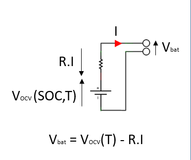
Charge |
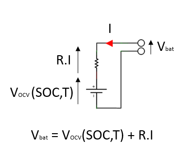
Discharge |
|
|
The model is assumed to be linear up to the "gassing" region and down to the deep discharge beginning.
The basic linear model takes the simple form :
Ubatt = Uocbase + Alpha · SOC + Beta · (Tbatt - Tref) + Ri · Ibatt
with: Ubatt = voltage for a battery- element.
Uocbase = intercept of the open circuit voltage linear part at SOC=0.
SOC = state of charge (varies from 0 to 1).
Alpha = slope of the open-circuit line (depends on the chemical couple Pb-SO4).
Tbatt = temperature of the battery.
Tref = reference temperature (usually 20°C).
Beta = temperature coefficient (-5 to -6 mV/°C).
Ri = internal resistance, assumed to be constant.
Ibatt = battery current (charge > 0, discharge < 0).
The values of the parameter, characteristic of the electrochemical Pb-H2SO4 couple, are drawn from a manufacturer's catalog.
This model is then completed by a series of disturbances, whose values are predefined in the program (modulated especially by the chosen technology), but which can of course be adjusted by the user if he has more specific data for his own battery at disposal.
The first two disturbances to be taken into account are the behaviours at the end of the charging and the discharging processes, which mainly affect voltage, and therefore regulation.
When the battery approaches complete discharge, the voltage falls progressively, whatever be the current. We have fixed a fall of a quadratic shape starting from a SOC of 30%, which gives realistic results for most of the batteries. But this exact shape is of little importance for the behaviour of the system as a whole.
At the end of charge, the problem is more delicate because of the apparition of the electrolyte dissociation ("gassing"). This phenomenon is rarely treated explicitly in the usual models, but it is still fundamental as it consumes a part of the charging current, and therefore affects the global operating of the system, in particular the real efficiency of the battery. We suppose that this phenomenon induces an excess voltage with respect to the linear behaviour depending on the SOC. The shape of this excess voltage is a predetermined "S"-curve, (ref.[22]). The "gassing" current increases exponentially with the excess voltage, and substitutes itself progressively for charge current. The "Delta" coefficient of the exponential has been measured by a German team for various batteries of different ages, and is established at about 11.7 V-1 (ref.[23]). The end of charge is another predetermined limiting curve, depending on the charging current (ref.[20]). It corresponds to the situation where the whole current is used for the dissociation, and allows to fix the Iogass parameter:
Igass = Iogass · exp ( Delta · dUgass).
To put it more simply, the dependence of the voltage on the temperature is assumed to be linear in all operating conditions. In the same manner, the internal resistance is assumed to be constant; any possible dependence on temperature (studied in ref.[21]) is ignored. We also neglect the polarisation effects, or voltage drift depending on immediately preceding operating conditions; they show characteristic times less than one hour, and only affect the states of very low current.
The state of charge remains to be determined. Fundamentally, it corresponds to the charging and discharging balance currents, with respect to the nominal capacity of the battery. But a number of corrections are to be made.
First, the electrochemical conversion (an SO4-- ion - 2 electrons of current) is not perfect: the balance, called " coulombic efficiency ", is of the order of 0.97 for the batteries usually used in solar installations. This efficiency can be specified by the user, but remains constant in all the conditions of use. It should not be mixed up with the global current efficiency, including losses from "gassing" current, which depends on the operating conditions and appears as a simulation result. The coulombic efficiency is applied to the charging current.
We then have the loss due to self-discharge current, which strongly depends on temperature, type and age of the battery. The temperature behaviour of the self-discharge current does not depend very much on the type of battery: it is close to an exponential, and doubles every 10°C. In the programme, it is specified by a predefined profile (which increases steeply for uses above 20°C). But its basic value at 20°C is asked in the module of the secondary parameters.
The modelling of the "gassing" current also allows for the calculation of the quantity of electrolyte consumed, giving an idea of the frequency of maintenance (distilled water checks and addition). Unfortunately - or fortunately! - the problem is not all that simple as some sealed batteries (said to be without maintenance) contain a catalyst which allows the recombination of H2 and O2 gases to again give water.