|
<< Click to Display Table of Contents >> Near Shadings: tutorial |
  
|
|
<< Click to Display Table of Contents >> Near Shadings: tutorial |
|
The near shadings are one of the most difficult parts of PVsyst. Therefore, here we present a full exercise to explain the main steps and tips/advices to use this tool easily.
This is built from the following "architect" plan:
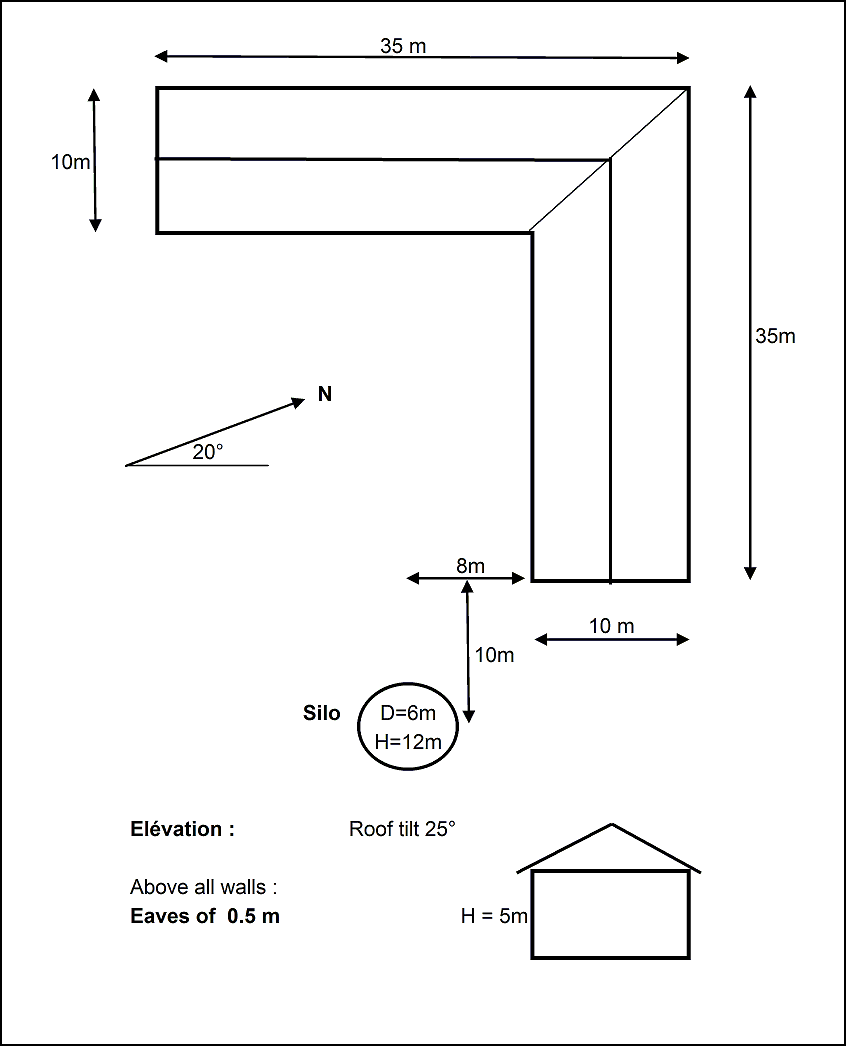
Defining the 3D scene:
- Open the button "Near Shadings" and then "Construction/Perspective".
You obtain the main 3D window where you will construct your "scene".
Constructing the building.
The building will be an assembly of elementary objects, gathered afterwards as one individual object in the main 3D scene.
- In the menu, choose "Create" / "Building/Composed object".
This will open a secondary 3D window, which is the referential of the building object.
- In the menu, choose "Add object".
Here, choose "Parallelepiped" and define the sizes (Width = 10m, Length = 35m, Height = 5m).
- Click "OK", this will place the parallelepiped in the building object's referential.
- In the menu, choose again "Add object".
Here, choose "Parallelepiped" and define the sizes of the second wing of the farm (Width = 10m, Length = 25m, Height = 5m).
- Click "OK", this will place the parallelepiped in the building object's referential, positioned at the origin.
Positioning in the 3D scene
You now have to position this second wing in the scene.
Please observe that to select an object, you have to click on its edges in Technical view and on anywhere on it in Realistic view. Objects are drawn in red when selected.
- Click the "Top View" button or press F3.
- Perhaps you want to diminish the scale ("Zoom backward" button).
- Perhaps you want to recenter your scene: click on the scene - but not on an object - and drag the scene's plane.
- Be sure that the positioning tool is activated (button with 4 crosses on the left). This opens the "Object positioning" dialog.
- Now, you can click and drag the red point to move the selected object with the mouse, and the violet point to change its orientation. Position and orientate the object roughly at its place as second wing, perpendicular to the first parallelepiped.
- The mouse does not allow to get accurate values. But after rough positioning, the dialog will give you the order of magnitude so you can finely adjust the exact values according to the architect's plans. In this case, you will put X = 10.00m, Y = 10.00m, and do not forget Azimuth = 90.0°.
NB: Please avoid the interpenetration of objects. This often creates problems for a correct shade calculation.
Now you have to add the roof.
- Main menu "Elementary Object" / "New object" and choose "Two-sided roof + Gables".
- Define the sizes: "Base width" = 11m, "Top length" = 30.5 m (for eaves), "Roof tilt" = 25°, and "Gable 1 angle" = -45°.
- Click "OK". This will put the roof in the building's scene. You can position it with the mouse and values as before (X = 5, Y = 5, and Z = 5, building heigth).
- For the second wing, you could do the same. You can also reuse this existing roof: "Edit" / "Copy", and "Edit" / "Paste". You will obtain a second instance of the selected object.
- Position this object by mouse and values (be careful with the new azimuth, exactly 90°).
Now, the 45° cut gable is not correct. To modify the selected object, you can:
- either choose "Elementary Object" / "Modify",
- or, more easy, double-click the object on its border.
- Change -45° to +45° and click OK.
Now your building is finished, you can include it in the main 3D scene through the menu "File" / "Close and Integrate".
Adding the PV plane
PV planes cannot be integrated in building objects, as the PV planes elements (sensitive areas) are treated differently in the program. They should be positioned on the building only within the 3D scene.
- In the main 3D scene, choose: "Object" / "New..." / "Rectangular PV plane".
- You have to define the sizes: "Nb of rectangles" = 1 (you could define several non-interpenetrating rectangles in the same plane), "Tilt" = 25°, "Width" = 5.5 m, "Length" = 25 m.
NB: There is no relation at this stage with the real size of the PV modules in your system definition. The program will just check at the end of the 3D definitions that the "plane" sensitive area is greater than the area of the PV modules defined in the system, without shape considerations.
- Click "OK". The plane comes with respect to the origin in the 3D scene.
- To position it, again click "Top view" and position it globally with the mouse. Now, you don't have rigorous references and you don't need to adjust the values, but be careful not to interpenetrate the other roof! Also, check the azimuth value (should be exactly 90°).
- Vertical positioning: now your field is on the ground. Click the oberver's "Front View" button, and position your plane on the roof by dragging the red dot with the mouse. Please always leave some spacing between any active area and other objects (minimum, say 2 cm). If you put the plane below the roof, it will obviously be shaded permanently !
Completing with the silo and a tree
- In the main scene: "Object" / "New..." / "Elementary shading object" / "Portion of cylinder". According to the plan: define Radius = 3m, Aperture angle = 360°, Nb of segments = 16, Height = 12m. Click "OK".
- In the main scene, be sure that the "Positioning" tool is activated, click "Top view" and position the silo with the mouse (if you do not know the order of magnitude or signs), and then with values (X = 18m, Y = 45 m).
- You can also put a tree in the courtyard. "Object" / "New..." / "Elementary shading object" / "Tree". To determine the sizes and shape of the tree, you can use "Front view", and here, play with the red points to adjust the shape of your tree. And then you position it as you like in the courtyard (please remember: a tree doesn't have definitive sizes!).
Positioning with respect to the cardinal points
For convenience, you construct the scene in the referential of the architect. After that, the button "Rotate whole scene" will perform the final orientation of the global scene.
- Select the reference object for the orientation (normally the PV plane).
- In the "Rotate Whole Scene" dialog, define the new azimuth (here +20°, west). This will orientate your whole scene. But each time you will have to re-position an object in the scene, it will be easier to come back in the original system's referential, i.e. to a plane orientation of 0° or 90° !
Shading test and animation
Now your 3D scene holds obstacles and sensitive area, it is ready for a shading analysis.
- Push "Shadow animation over one day" button. And in this tool "Play/Record animation". The shadows will be shown for the whole selected day. After execution, you have a scrollbar to review one or the other situation.
For each time step, the date/hour, sun position and shading factor are mentioned on the bottom of the 3D window. You can try this for different dates in the year.
If there is some shade that you don't understand well, you can click the button "View from the sun direction" on the top group. This way you will have a direct view of the shades and their cause.
Colours
You can now personalize the view of your scene by defining colours.
- Click the 9th button from the left "Realistic view".
- The colour of each element may be defined in its definition dialog.
- For example for the building: Double-click the building, this will open the building construction.
- Double-click the roof, this will open the definition dialog.
- Here you can define the colour of the roof, and the colour of the gables independently.
- Please note: the colours are defined "at bright sun": choose them rather light.
- If you define your own colours, store them as "personalized colour" in order to reuse them for other similar objects.
Recording the scene
If you do some bad manipulation, you have the possibility to Undo (2nd button left).
As the 3D tool is not fully safe in PVsyst (sorry... this is not easy to program and there are still some bugs), and you can also do bad manipulations, you are advised to periodically save your shading scene using "File" / "Save scene" as a *.shd file.
Please note: your definitive scene (used in the simulation) will be stored along with your "MyProject.VCi" file. It doesn't require a *.SHD file.
Display in report
This scene will appear on the final report. If you want to have a specific view of the scene in the report, you can request it by "File" / "Save scene view" / "Keep this view for the report".
Use in the simulation
Now, your shading scene seems to be ready for the simulation.
- Choose "File" / "Close". You return to the near shadings dialog.
- Choose "Linear shadings" in the box "Use in simulation".
Here, the program checks the compatibility of your 3D scene with the other definitions of your system.
| - | The plane orientation should match the one defined in the "Orientation" part. If not, you have a button to eventually correct the "Orientation" parameters according to the 3D construction. |
| - | The sensitive area should be sufficient to position the PV modules defined in your system definitions. This is a rough test that checks only the area, not according to the real sizes and geometrical positioning of your modules. The maximum area value for warnings is much higher, to account for installations with spaced modules. |
| - | When everything is correct, the program asks to compute the Table of the shading factors. |
The table is a calculation of the shading factor (shaded fraction of the sensitive area, 1 = no shadings, 0 = full shaded), for all positions on the sky hemisphere "seen" by your PV plane. It allows the calculation of the shading factor for the diffuse and albedo (which are integrals of this shading factor over the concerned spheric portion). At each hour, the simulation process will interpolate in this table - according to the sun position - to evaluate the present shading factor on beam component.
This also allows the construction of the iso-shadings graph, that gives a synthetic view of the time in days and seasons where the shadings are problematic. The line 1% for example, gives all the sun's positions (or time in the year) for which the shading loss is 1%, i.e. the limit of shadings.
Now clicking "OK" will integrate this shading effect in the next simulation. In the final loss diagram on the report, you will have a specific loss for the "Near shadings".
Electrical effect: partition in module strings
Now when a cell is shaded, the current in the whole string is affected (in principle the current of the string is the current in the weakest cell). There is no possible accurate calculation for this complex phenomenon in PVsyst. We will just assume that when a string is hit by a shade, the whole string is considered "inactive" concerning the beam component. This is an upper limit on the shading effect: the truth should lie between the low limit - which we call the "Linear shading" - representing the irradiance deficit, and this upper limit (see partition in module strings), representing the electrical effect.
For this second simulation "According to module strings":
| - | Go back to the Near Shadings definition, button "Construction/Perspective" |
| - | Click the button "Partition in module chains" on the left. |
| - | Here you can split the field into several equivalent rectangles, each representing the area of a complete string (not a module !). If several subfields, you should do this for every subfield rectangle. |
This is a rough estimation, for a rough computation. Perhaps you will not be able to represent the real arrangement of your modules. But you can try different configurations, perform the simulation and then decide which configuration is the best suited for your particular system.
| - | When performing the shading animation, the partially shaded rectangles will now appear in yellow. The new shading factor is the sum of the grey+yellow areas, with respect to the field area. |
Use in the simulation
| - | In the same way as before, in the "Near shadings", please choose "According to module strings" in the options "Use in simulation". |
| This will ask for computing the tables, and then you can open the iso-shading graph for comparing the effect to the "Linear" one. |
| - | "Fraction for Electrical effect": this is the way how the yellow parts will be treated in the simulation. A 100 % value will withdraw the total electrical production of these areas in the simulation. This is the upper limit of the shading effect. Perform a simulation with this value. |
| - | For the simulation presented to you end-customer, you can fix a different value for better approaching the reality. But sorry in the present time we don't have means for a good estimation of this factor (perhaps around 60-80%, accounting for the by-pass diodes partial recovery ???). |
Horizon (far) and near shading cumulation
During one step of the simulation, the program will first evaluate the beam component according to the horizon line (ON/OFF, full or zero), and then apply the near shadings factor on the beam component.
Therefore, when the sun is below the horizon line, there will be no near shading loss as the beam is null. In other words, potential near shadings for sun positions already concerned by horizon will not produce any additional losses.