Backtracking performance
In tracking arrays, mutual shading can be significant near sunrise and sunset. Adopting a backtracking strategy often improves the system yield for a fixed GCR at a given location. However, the gain compared to standard tracking depends on tracker type, location, climate, terrain, panel type, etc. We advise to compare yields for both tracking and backtracking scenarios, especially when working with an uneven terrain.
Comparing performance
When comparing the yields of a given installation with or without backtracking, it is important to use the right metric. It is advised to not use the Performance Ratio (PR). The PR does not account for the cosine effect, as explained here. It is preferable to use the Specific Production (also called Specific Yield) instead.
Yield comparison on ideal system
The graphs below show the energy yield as a function of GCR for different Horizontal Single-Axis Tracker (HSAT) systems of 400 kWp (STC) each. All scenarios are simulated for a perfectly regular flat array with a N-S tracking axis; shadings are simulated using the module layout option. The different systems considered are:
- Different tracker layouts: 1 module in landscape (1L) or 4 modules in landscape (4L)
- Monofacial or bifacial panels
- Different locations: Copenhagen (Denmark) and Nairobi (Kenya)
| Monofacial panels | Bifacial panels |
|---|---|
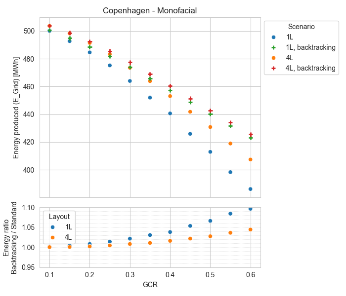 | 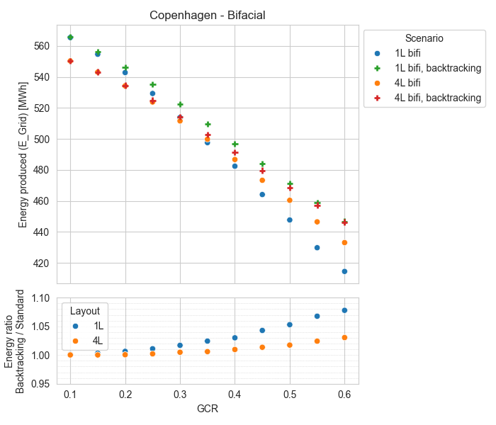 |
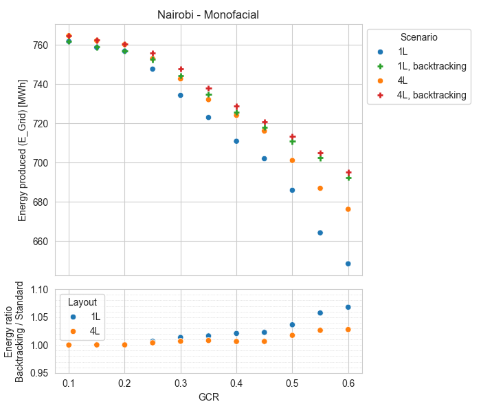 | 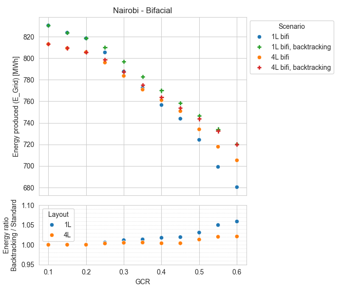 |
In these flat and regular scenarios, using a backtracking approach instead of standard (astronomical) tracking makes little difference at low GCR, and always improves the yield for denser tracker layouts. The gain depends on the system considered, as follows:
- The gains from backtracking are greater for the 1L system than for the 4L system. This is expected because, when using standard tracking, the losses are higher with a one-module tracker (as no module remains unshaded), and losses decrease as the number of module rows increases.
- The gain from backtracking is lower for bifacial systems (no optimization for rear-side irradiance).
- The gain from backtracking is lower in Nairobi, Kenya (low latitude) compared to Copenhagen, Denmark (high latitude, more diffuse light).
Please keep in mind that results may differ in more complex layouts. Irregular terrain or irregular tracker positioning may still lead to mutual shading or sunlight strips reaching the ground, reducing the effectiveness of a backtracking approach.
Understanding losses
The losses in backtracking and non-backtracking systems are different. This is illustrated in the example below.
The system considered here is a Horizontal Single-Axis Tracker (HSAT) with a N-S axis in Santiago (Chile). The phi angle limits are ±60°, with four rows of modules in landscape orientation across the tracker width.
- With backtracking, the losses due to misorientation are slightly lower than the "linear" shading losses without backtracking (irradiance deficit, including diffuse, but ignoring electrical mismatch).
- The electrical losses + IAM without backtracking are very similar to the losses due to albedo and diffuse shading + IAM with backtracking.
- It is notable that with backtracking, the loss from diffuse light diminishes while IAM increases at high GCR, due to the tracking angle limitations imposed by backtracking. Both effects compensate each other.
![]()