Heat transfer coefficients (U-values)

The heat transfer coefficients \(U_c\) and \(U_v\) described in the definition of the steady-state thermal model $$ \begin{equation} T_{\mathsf{SS}} - T_{\mathsf{amb}} = \dfrac{\alpha G (1 - \eta)}{U_c + U_v W_s}. \end{equation} $$ are the main input parameters defining the PV array thermal behavior. As can be seen, the heat exchange is split into two components: a constant component and a factor proportional to the wind velocity. \(U_c\) and \(U_v\) are the conductive and convective heat transfer coefficients, more commonly called "U-values", and are expressed in \(\left[\frac{\mathrm{W}}{\mathrm{m^2K}}\right]\) and \(\left[\frac{\mathrm{Ws}}{\mathrm{m^3K}}\right]\), respectively.

These values need to be determined empirically by fitting equation (1) to real system data.

U-values fit to measurements

Fitting the U-values to real PV system measurements requires long-term data acquisition on site (typically several months with 5-10 min or hourly values), in order to gather data covering a sufficient range of meteorological conditions. These measurements are performed on the PV array in operation.

The required measurements are:

• The incident irradiance on the collector plane (POA or GlobInc value).

• The ambient temperature should be measured in conditions as close as possible to those of the weather data used in the simulation. Per WMO-No. 8 (CIMO Guide, Chapter 2)¹, the sensor should be installed 1.25–2 m above the ground, over natural ground, and shielded from direct solar radiation by a screen or shield. It should be positioned away from large heat sources such as concrete surfaces or buildings.

• The PV array backside temperature, as a proxy for the solar cell temperature. Note that for equation (1) to represent accurately the solar cell temperature, the isolation conditions of the temperature probe need to be considered carefully², as there can be a difference of \(0\) to \(3 ~\mathrm{°C}\) between the solar cell and PV module backside³.

• Possibly the wind velocity (measured in the same conditions as the values that will be used during the simulation, which are typically measured at \(10 ~\mathrm{m}\) above ground).

Then, the slope of the distribution of \((T_{\mathsf{SS}} - T_{\mathsf{amb}})\) as a function of irradiance is related to the heat transfer coefficients.

When no wind velocity data are available, the slope gives a single coefficient \(U_c \equiv U\) that embodies both the constant conductive heat exchange and an average convective heat exchange corresponding to the site's average wind velocity.

With wind velocity measurements, the treatment is more complex and involves a bilinear fit. We intend to develop a dedicated tool for such analysis in a future version of PVsyst.

Example

Here is an example of a one-year measurement on a PV array of frameless modules, mounted with an \(8 ~\mathrm{cm}\) gap on a quasi-horizontal steel roof, with some spacing between module rows.

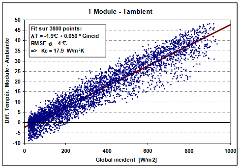
The linear regression gives a value of \(-1.9 ~\mathrm{°C}\) for the intercept at \(\mathrm{GlobInc} = 0\), and a slope of \(0.05 ~\frac{\mathrm{Km^2}}{\mathrm{W}}\).

From expression (1), we easily deduce that $$ U = \frac{\alpha (1-\eta)}{\mathrm{Slope}} $$

This was an amorphous system with an average efficiency of the order of \(5 ~\%\), and the slope was evaluated without the intercept of \(-1.9 ~\mathrm{°C}\), i.e. \(0.048 ~\frac{\mathrm{Km^2}}{\mathrm{W}}\), leading to a value of the heat transfer coefficient \(U = 17.9 ~\frac{\mathrm{W}}{\mathrm{m^2K}}\).

Note: on this graph, we observe temperature differences (TArray - TAmb) below 0 at low irradiance. This is explained by the infrared exchange deficit under clear-sky conditions. The PV array emits infrared radiation according to its temperature. This emission is counterbalanced by the emission of the ambient environment. When the weather is cloudy, the ambient IR is produced by the nearby air. But under clear-sky conditions, the IR is emitted from the higher layers of the atmosphere, which are at lower temperatures. This may explain temperature differences of several degrees.

Discussion

We discuss here several potential sources of artifacts when establishing the U-values from measurements, as well as caveats regarding their generalization to other systems. There is no simple physical model for estimating the U-values in the general case. The only reliable way to determine this parameter is to measure it on site.

The U-values depend on the module mounting mode (fixed tilt, roofing, facade, trackers, floating systems, concrete floor or grass, etc.), which affects the thermal exchange of the PV array with its environment.

For example, with free air circulation all around the tables (i.e. PVtables in row arrangements), these coefficients are affected by heat transfer on both sides of the PV module. If the back of the modules is more or less thermally insulated, the coefficients should be lowered, theoretically down to half the value when the back side is fully insulated (i.e. it no longer participates in thermal convection and radiation transfer).

All the physical phenomena not described by equation (1), such as radiative heat exchange or absorption on the rear side, are effectively included in the fitted coefficients. However, to reapply these coefficients to another system, one should make sure that the second system resembles as closely as possible the original system on which the coefficients were fitted.

A similar caveat is that the ambient temperature and wind speed used during the simulation need to be measured in exactly the same way as they were on the original system. According to meteorological standards, wind velocity should be measured on a mast at a height of \(10 ~\mathrm{m}\) in a free environment. This is rarely the case when wind velocity is measured for PV system monitoring. The real value at the collector level may be lower by \(35\) to \(50 ~\%\). Therefore, the wind parameter \(U_v\) should be adapted to the way the wind velocity is recorded. Due to this source of ambiguity, PVsyst does not provide a default \(U_v\) value at present. Instead, we propose a default value for \(U_c\) that includes, on average, the effect of wind speed.

Default and proposed values

In the absence of reliable measured data, PVsyst proposes default values without wind dependency (i.e. assuming an average wind velocity):

• For free-standing (open-rack) systems, i.e. with air circulation all around the collectors, according to our measurements on several installations:
  • \(U_c = 29 ~\frac{\mathrm{W}}{\mathrm{m^2K}}, \quad U_v = 0 ~\frac{\mathrm{Ws}}{\mathrm{m^3K}}\)
• Therefore for fully insulated backside (no heat exchange at the backside, only one side contribution to the convecting heat exchange), the \(U\) value should be divided by 2:
  • \(U_c = 15 ~\frac{\mathrm{W}}{\mathrm{m^2K}}, \quad U_v = 0 ~\frac{\mathrm{Ws}}{\mathrm{m^3K}}\)
• For intermediary cases (semi-integration, air duct below the collectors), the value should be taken between these 2 limits, but preferably lower than \(22 ~\frac{\mathrm{W}}{\mathrm{m^2K}}\), as air heat removal is often not very efficient. The default value proposed by PVsyst for any new project is
  • \(U_c = 20 ~\frac{\mathrm{W}}{\mathrm{m^2K}}, \quad U_v = 0 ~\frac{\mathrm{Ws}}{\mathrm{m^3K}}\)
  • We have chosen this value as a general default because we consider it more representative of usual rooftop systems, managed by users who will not necessarily modify the PVsyst default. For large systems, we assume that trained engineers will adjust this parameter accordingly, for example to \(29 ~\frac{\mathrm{W}}{\mathrm{m^2K}}\) for row-like large power plants.
• For domes, a manufacturer has measured the U-value on several installations (height about \(40\) to \(70 ~\mathrm{cm}\) above the ground):
  • \(U_c = 27 ~\frac{\mathrm{W}}{\mathrm{m^2K}}, \quad U_v = 0 ~\frac{\mathrm{Ws}}{\mathrm{m^3K}}\)

Now, if reliable hourly wind velocity data are present, we cannot propose a "universal" \(U_v\) value. It would depend on many parameters, and especially on the way this wind velocity is measured. PVUSA proposes the following thermal correlation, widely used for the free-standing (open-rack) situations when wind speed data are available from official climatic data:

• \(U_c = 25 ~\frac{\mathrm{W}}{\mathrm{m^2K}}, \quad U_v = 1.2 ~\frac{\mathrm{Ws}}{\mathrm{m^3K}}\)

This corresponds to our default \(29 ~\frac{\mathrm{W}}{\mathrm{m^2K}}\) when the average wind velocity is \(3.3 ~\mathrm{m/s}\), which is rather usual in continental, non-coastal situations.