Steady state thermal model

Steady-State Thermal Balance Model

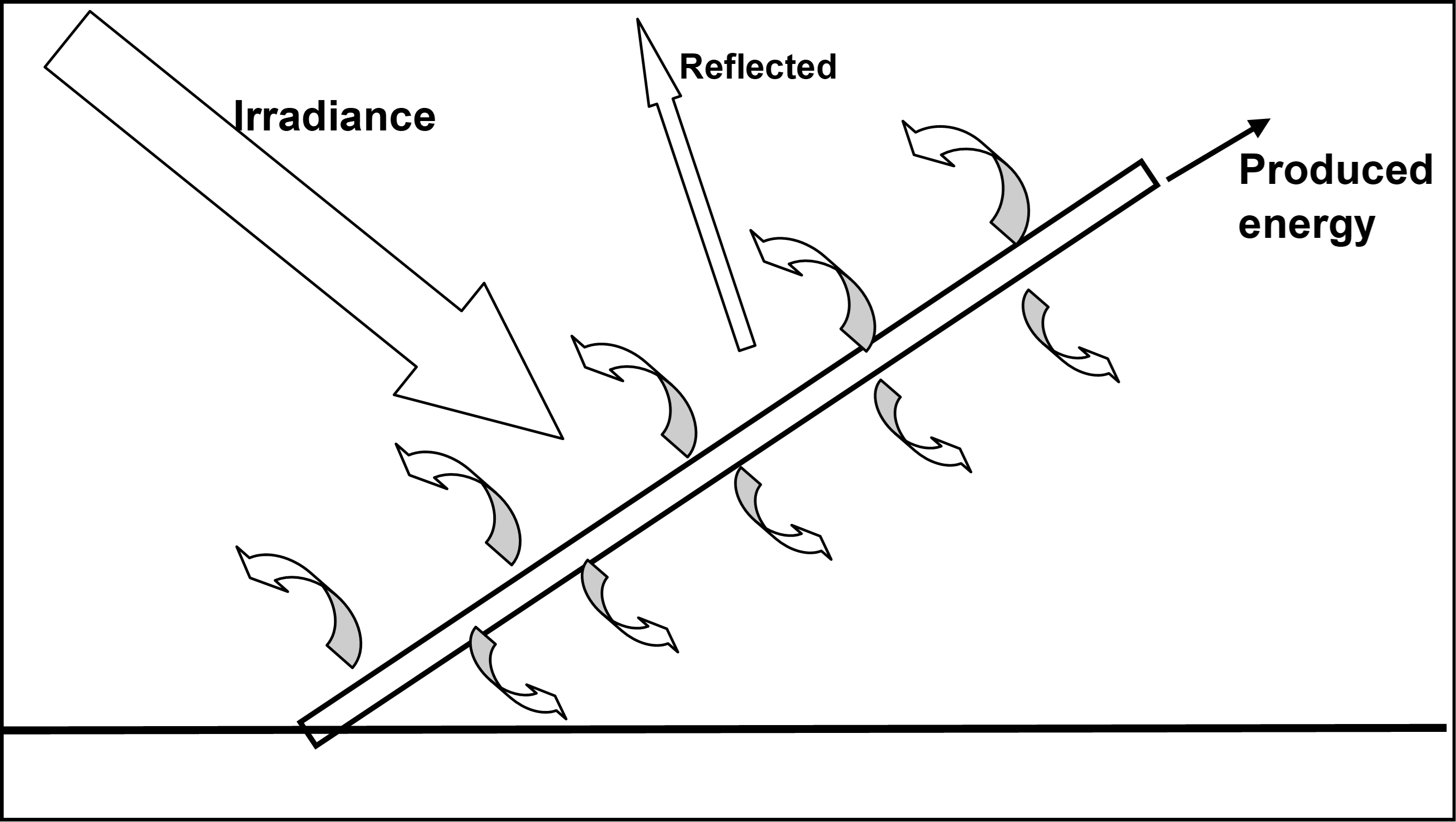
First, the thermal balance model is used to evaluate the steady-state temperature of the PV array, i.e. the average temperature the PV array would reach if the external conditions were fixed for an infinite time. The balance is based on the incident irradiance absorbed by the modules, the heat emitted back to the environment, and the extracted electrical power.

PVsyst models this energy flux balance with the following equation:

\[ \begin{equation} \alpha G (1-\eta) = (U_c + U_v W_s)(T_{\mathsf{SS}} - T_{\mathsf{amb}}) \end{equation} \]

where the different parameters are defined and explained below:

The heat exchange is split into a constant component and a factor proportional to the wind velocity. $U_c$ and $U_v$ are the conductive and convective heat transfer coefficients, more commonly called "U-values", and are expressed in $\left[\frac{\mathrm{W}}{\mathrm{m^2K}}\right]$ and $\left[\frac{\mathrm{Ws}}{\mathrm{m^3K}}\right]$, respectively. They determine the heat flux as proportional to the temperature difference between two media. The U-values must be fitted to real system data, as discussed here.

$\alpha$ is the absorptance of the PV module at normal incidence, i.e. (1 - reflection - transmittance). By default, we consider the value $\alpha = 0.9$, corresponding to a rough evaluation of the reflection losses at normal incidence at the air/glass interface. Given that mainstream PV modules have very similar reflectance and very often zero transmittance, any inaccuracy in our choice of $\alpha$ will be balanced out in the fit of the U-values. However, for PV modules with atypical reflectance, it is possible to modify the $\alpha$ value in the .PAN file menus, although this is recommended only for very special PV modules.

$G$ is the incoming irradiance on the PV module surface. During the simulation, this value is the effective irradiance on the PV array, i.e. the PVsyst variable GlobEff, which takes into account the losses of irradiance due to shading and to the enhanced reflection at non-normal incidence. In contexts where these are not defined, the irradiance in the plane of array is used instead, i.e. the PVsyst variable GlobInc.

$\eta$ is the PV module efficiency and is used here to calculate the electrical energy removed from the module. As $\eta$ itself depends on temperature, several iterations are needed to compute the temperature; see below.

$W_s$ is the wind speed in $\left[\mathrm{m/s}\right]$ read from the weather data, usually measured at $10 ~\mathrm{m}$ above ground.

$T_{\mathsf{amb}}$ is the ambient temperature read from the weather data.

$T_{\mathsf{SS}} $ is the PV array steady-state temperature, i.e. the PVsyst variable TArrSS.

PV module vs Cell Temperature

The heat balance equation (1) implicitly assumes a very thin PV module. In this approximation, there is no distinction between the temperature of the PV cell and the temperatures of the PV module surfaces.

In practice, however, a thermocouple placed on the back of a PV module can measure a difference of $0$ to $3 ~\mathrm{°C}$ compared to a direct measurement of the PV cell temperature¹. Nevertheless, this small difference is difficult to distinguish from measurement artifacts (e.g. the thermal isolation conditions of the thermocouple²); it depends on the installation context (open-rack vs. dome or rooftop PV, installation over concrete or grass, etc.), and it has little impact on PV production (< $0.5 ~\%$). Therefore, it is justified to work with this approximation.

Iterations between temperature and efficiency

Equation (1) can be rearranged to give the PV array temperature as a function of the other variables:

\[ \begin{equation} T_{\mathsf{SS}} = T_{\mathsf{amb}} + \dfrac{\alpha G (1 - \eta)}{U_c + U_v W_s}. \end{equation} \]

However, the PV module efficiency $\eta$ computed by the PV electrical model is also a function of temperature. We treat this recurrence differently depending on the context:

Within the simulation, we compute temperature and efficiency iteratively, starting with an initial efficiency of $20 ~\%$. In most cases, $2$-$3$ iterations are sufficient to reach an accuracy below $0.1 ~\mathrm{°C}$.
Outside the simulation, in specific tools where the PV module electrical model is not defined, we perform a single computation assuming an efficiency of $20 ~\%$, which is reasonable for modern PV modules.

David L. King, William E. Boyson, and Jay A. Kratochvil. Sandia model- photovoltaic array performance model. Technical Report, Sandia National Laboratories, Photovoltaic System R&D Department, Albuquerque, New Mexico 87185-0752, 2004. SAND2004-3535 report, Unlimited Release, August. ↩
Kensuke Nishioka, Kazuyuki Miyamura, Yasuyuki Ota, Minoru Akitomi, Yasuo Chiba, and Atsushi Masuda. Accurate measurement and estimation of solar cell temperature in photovoltaic module operating in real environmental conditions. Japanese Journal of Applied Physics, 57(8S3):08RG08, August 2018. URL: https://iopscience.iop.org/article/10.7567/JJAP.57.08RG08 (visited on 2025-04-14), doi:10.7567/JJAP.57.08RG08. ↩